Case study

Transport properties

Liquid Argon

In the following tutorial, we are going to show you how to compute the self-diffusivity ($D$), dynamic viscosity ($η$), isochoric heat capacity ($C_v$), and thermal conductivity ($k$) of 512 liquid Argon atoms at ~85 K and 1 atm.

The tutorial consists of 4 stages:
1) Initializing and equilibrating the atomic positions of a liquid Argon system.
2) Setting the temperature and the pressure to ~85 K and 1 atm.
3) Running long run dynamics simulation so that transport properties can be measured.
4) Measuring $D$, $η$, $C_v$, and $k$.

Section 1. Initializing and equilibrating

Video 1. Section 1 summarized into a 2 minute video. For a detailed explanation, follow the tutorial below.

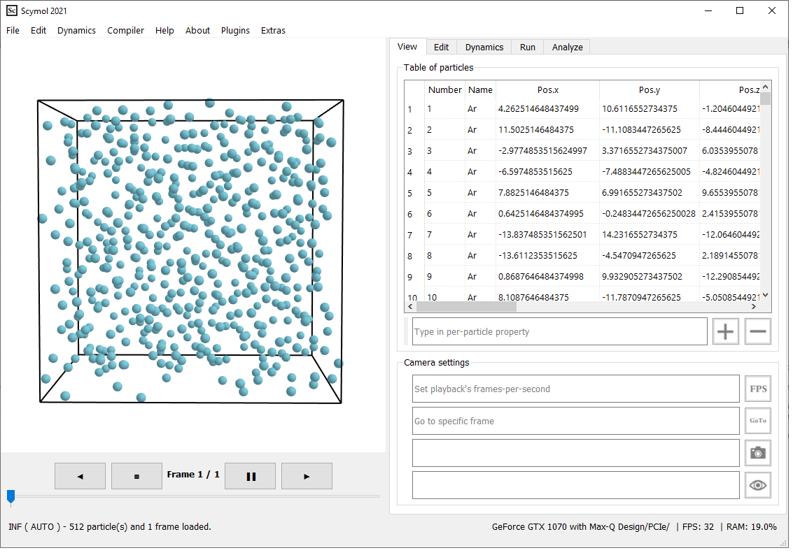
1.1 Launch Scymol. If you have not set it up yet, please refer to scymol.com/get to download, set up, and launch Scymol.
1.2 Open the Build window. The Build window will allow us to create an atomic model containing the Argon atoms.
1.3 Load an Argon atom. Click on the Plus sign and select Import when the context menu appears. Navigate to Scymol\structures\periodic_table and double-click on the Ar.csv file.
1.4 Create a liquid Argon pool. Once the Argon atom is loaded, input the number of particles ($N = 512$) in the Number of replicas input box. You can ignore the Random rotation checkbox as single atoms molecules are not rotated. In the Dimensions section, select the Side length option from the dropdown menu and type '28.96' in the input box right next to it. The density of liquid Argon at 85 K and 1 atm is approximately $\rho \approx 1400 Kg/m3$. This means that in order to build a box that contains $N = 512$ atoms with a density of $\rho \approx 1400 Kg/m3$, the cubic box's side length ($L$) should be ~28.96 Å. The formula used to compute the side length is: $$L=\sqrt[3]{\frac{N\times M}{{\rho N}_{av}}\ ,}$$ where $N$ is the number of particles, $M$ is the average molecular weight of the molecule or atom, $\rho$ is the mass density, and $N_{av}$ is Avogadro's number. You can also choose the Density option in the drop down menu and type in '1400'.
Select the Sobol option in the drop down menu of the Distribution function section. This setting allows Scymol to distribute the particles using a low discrepancy random distribution function Distribution of points in a cube and approximate evaluation of integrals. https://doi.org/10.1016/0041-5553(67)90144-9 so that the particles overlap the least possible and are distributed as evenly as possible within the cubic box. By doing this, we save some time when trying to equilibrate particle positions by initially placing the particles in a lower energy configuration.
Click on the Build button on the bottom right. The atomic system should appear in the 3D section of Scymol, and should look very similar to the one portrayed in Figure 1.

**Figure 1.** Liquid Argon system created using Scymol's *Build* tool. Atomic positions are generated using a Sobol sequence, a low discrepancy statistical method that distributes the particles in 3D uniformly (i.e., preventing overlapping).

Even though you set the density or the bounding box's size to a value, the particles are still randomly distributed and may not occupy positions so that the bounding box's dimension perfectly matches the dimensions desired. It is very important to force set the box's dimensions so that $L = 14.48 Å$ (exactly). Go into the Dynamics→Boundaries tab, and type in $-L$, $L$, $-L$, $L$, $-L$, and $L$ in the input boxes in the Box dimensions section. Click on the check button at the bottom left so that the changes are applied.
1.5 Force field input and parameters. Now that we have the pool of liquid Argon atoms, we have to define the forces that are going to influence our system. Liquid Argon is a very simple fluid, and can be modeled accurately by just using a Lennard-Jones potential that represents Van der Waals interactions. This is because Argon forms no bonds (hence no bond, angular, or torsional strains are present) and it holds no partial or formal electric charge. The Lennard-Jones potential is given by $$E\left(r\right)=4\epsilon\left[\left(\frac{r}{\sigma}\right)^{-12}-\left(\frac{r}{\sigma}\right)^{-6}\right]\ \ ,$$ where $r$ is the interatomic distance between two atoms, $\sigma$ is the equilibrium distance, and $\epsilon$ is the lowest point in the energy well of the potential. Go into the Dynamics→Potentials tab, and enter the Lennard-Jones potential into the input box inside the Type 2 interaction category (You can copy/paste the following line directly into Scymol).

4*eps*((sigma/r)**12-(sigma/r)**6)

For more information on how force fields are derived and entered into Scymol, refer to Theory. Also, make sure that the fields for Type 1 forces are all set to 0.
Scroll down to the Force field interaction parameters section. In this part of the program, we input the parameters that govern specific atomic interactions. The value of the input parameter epsilon ($\epsilon$) in the Lennard-Jones potential, for example, changes with the nature of the atomic pair that is being computed. In our case, we only have one type of interaction possible (i.e., one possible atomic pair): one of an Argon atom that interacts with another Argon atom (Ar—Ar). The force field parameters for liquid Argon can be easily found in literature. One of the most used set of parameters in liquid Argon simulations are those estimated by Rahman Correlations in the Motion of Atoms in Liquid Argon. https://doi.org/10.1103/PhysRev.136.A405 , where $ \epsilon = 120.0 K$ and $ \sigma = 3.40$ Å. The value of $\epsilon$ has to be multiplied by $k_b$ so that we have it expressed in terms of energy units. Therefore, $$\epsilon = 120.0 \ K \times 0.831036 Å^2Da/ps^2/K = 99.72 \ Å^2Da/ps^2$$ We also have to define the maximum interaction distance ($R_{cut}$) beyond which the solver neglects any interaction; we do this to save computation time as the Lennard-Jones' potential energy tends to zero with distance rather quickly. For more information refer to scymol.com/numerical-methods. An interaction distance of $R_{cut}=2.5\times\sigma $ is often the rule of thumb used to truncate Lennard-Jones interactions. In our case, we are going to be slightly more conservative and set $R_{cut} = 11$ Å. Fill the values of $\epsilon$, $\sigma$, and $r_{cut}$ into the Type 2 and 3 table.
We must proceed to limit the magnitude of the forces (and energies) that are present between atomic pairs. This limitation must be set to readjust unusually high potential energy values resulting from certain atomic configurations. Scymol allows us to define an additional parameter, called $F_{2,Cap}$ so that we can initialize it to a value and set a cap, or a limitation, on the magnitude of the forces that result between the particles; any magnitude larger than the set cap would be forcibly set to the limiting value. Type in 'F2_Cap' in the Add property... input box and click on the Plus sign to add it. Initialize it to $F_{2,Cap} = 1\times10^4$. The general idea is that we run a series of simulations with increasingly large force caps so that eventually we reach a point where the particles have occupied lower energy positions and the force cap is no longer needed. We tell Scymol to increase the value of $F_{2,Cap}$ at each integration step. By using a semi-colon (;), we can add another statement into the Type 2 forces' formula as such:

4*eps*((sigma/r)**12-(sigma/r)**6); F2_Cap = F2_Cap + 50

Go into the Solver tab. Many liquid Argon simulations use an integration step $\tau_{step}$ that ranges between $\tau_{step}=5\times10^{-4}$ and $\tau_{step}=3\times10^{-3}$. We are going to choose $\tau_{step}=1\times10^{-3}$ for Equilibration stages. Type this value into Scymol's Integration step input box.
We are almost ready. We just need to navigate into the Run tab and set the number of cores that are going to be used. It is logical to think that the job will be finished faster if the core count is higher, and in most cases this is true. However, data communication and synchronization between the cores is also a computationally expensive task and for simulations with a relatively small $N$ and an unusually large assigned core count, the CPU will spend more time synchronizing data than computing it. For 512 particles, you are going to assign the maximum number that you can (depending on your computer) that is less than or equal to 12 cores. This is done by choosing a core count in the Parallelization section's drop down menu.
We now choose for how long is this stage of the simulation going to run. For this stage, 100 ps should be enough. Go ahead an type '100' in the Integration time step input box. The number of trajectories saved in this stage is unimportant; we are not going to be measuring properties in this part of the simulation. Save 5 trajectories if you want to exactly replicate the simulations run in the Case study. Once you type these into Scymol, click on Run. The simulation should take around 1 or 2 minutes to complete on a modern laptop.
After the simulation has finished, we have to make sure that we remove the energy/force limitation imposed and run the simulation again without it. Go back into the Dynamics tab and remove the additional statement that updates $F_{2,Cap}$ and also the parameter in the Type 2 and 3 forces table by clicking on the Minus button. Then, go into the Run tab and click on Run. The simulation should finish just fine; we are now ready to go to Section 2 of the tutorial.

1/4