Theoretical background
Code
The following section explains how Scymol is structured, which libraries it uses, how Python and Coarray Fortran (CAF) interface together, and how parallelization is achieved to run Molecular Dynamics (MD) simulations.
Structure
Scymol is divided into two sections. Section 1 corresponds to the simulation engine, responsible for all the calculations that occur in MD computations. It is written in CAF for computational efficiency, and compiled using OpenCoarrays every time the user submits a new calculation. Section 2 runs all the general purpose code, the graphical user interface (GUI) (built using PyQT5), the 3D environment (rendered with PyOpenGL), and Scymol’s data processing and plotting tools (using NumPy, SymPy, and Matplotlib).
Scymol's Section 2 is entirely written in Python3 due to its ease of use, universal support, and open source availability of a plethora of useful libraries. Python3 is however
an interpreted language, and lacks in performance against other classic, compiled languages such as C or Fortran. This is not an issue for Section 2, as it is not the part of Scymol
that performs heavy numerical calculations.
The GUI of Scymol is built using PyQT5.
Parallelization
Scymol allows the user to run MD calculations in parallel to take advantage of several computing cores to save time. CAF achieves this by independently executing an exact copy of the code on each available core. Each copy has its own set of data objects and is termed as an image. Images also have access to other images' information, meaning that any progress made by one image could (and sometimes must) be shared or synchronized with other images. In computational terms, Scymol follows a Single-Program-Multiple-Data (SPMD) programming model (See Figure 1). CAF has native support for both shared or distributed memory spaces, meaning that jobs submitted using CAF can run in single core laptops, as well as in multiple core computer clusters.
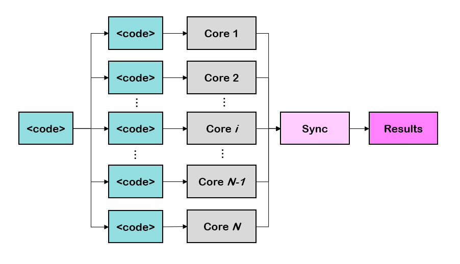
Figure 1. CAF uses a SPMD programming model to achieve multicore parallelization. In other words, parallelization is achieved by independently executing an exact copy of the code on each available core. CAF allows for data synchronization between ongoing tasks.
Scymol's parallelization technique works by assigning each available core an equal number of particles. This concept is explained thoroughly in the following paragraphs.
Let us start by creating a simple script that squares the elements of an array A=(1,2,3,4) running on just 1 core (i.e., it runs serially).
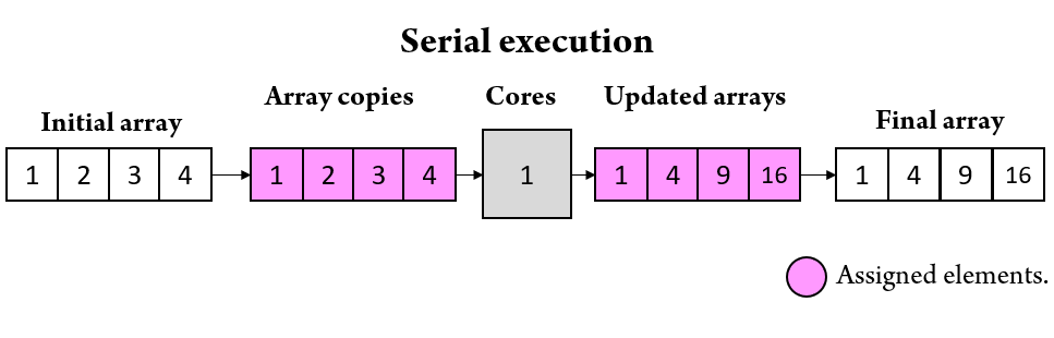
Figure 2. Visual representation of how a simple script would square the elements of an array if no parallelization scripting is applied.
program squares
implicit none
integer, parameter :: length = 4
integer :: A(length) = (/1,2,3,4/)

do i=1,length
	A(i) = A(i)**2
end do

print*, A
!Should print A = 1, 4, 9, 16.

end program squares
Code 1. Fortran script that squares the elements of an array A=(1,2,3,4).
Notice how the algorithm in Code 1 iterates over all the elements in A=(1,2,3,4). The code is essentially running on one core, and no work distribution or parallelization code is required. Now, let us assume that we are running the same script but written in CAF with the intent of distributing the work among two CPU cores. If we were to leave Code 1 untouched, CAF would simply execute two independent copies of the same script, each squaring all the elements in A. However, the objective is to distribute the work equally among every core available. This is visualized in Figure 3.
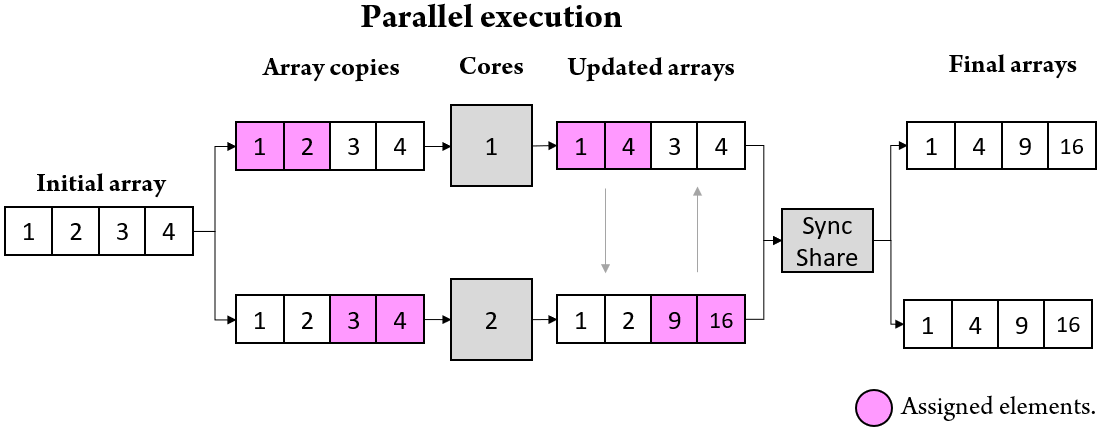
Figure 3. Visual representation of how the script from Figure 2 would run if its algorithm were to be parallelized using two cores. Cores #1 and #2 are assigned an independent copy of A
and a set of particles.
•Core #1 🠖 A(1:2) = 1,2
•Core #2 🠖 A(3:4) = 3,4
Each core proceeds to square their assigned elements on their copy of A and wait until all the other cores have finished. Local copies of A are then combined in
a data distribution step to form a resulting array containing every one of its elements squared.
One important step in writing parallelized scripts is the one responsible for cores' work synchronization and data distribution. Synchronization is important to force CPU cores not to overtake other cores, preventing race conditions. In CAF, the Sync All function forces CPU cores to wait for other cores before proceeding with any execution of code. CAF natively supports accessing or writing information among CPU cores by using brackets in addition to regular Fortran array notation (e.g., ARRAY(:)[core1]). Refer to Coarray Fortran's authors article: https://link.springer.com/referenceworkentry/10.1007%2F978-0-387-09766-4_477 https://doi.org/10.1007/978-0-387-09766-4_477. to read more about Coarray Fortran and the way it works.
program main
implicit none
integer, parameter ::  length = 4
integer :: i, low, high
integer :: A(length)[*] = (/1,2,3,4/)

low = (length*(this_image()-1)/num_images())+1
high = length*(this_image())/num_images()

do i=low,high
	A(i)=A(i)**2
end do

!Synchronization step:
sync all
do i=1,num_images()
	if (this_image() /= i) then
    	A(low:high)[i] = A(low:high)[this_image()]
	end if
end do
print*, A
!Should print A = 1, 4, 9, 16.

end program main
Code 2. CAF script that squares the elements of an array A=(1,2,3,4). Notice how the script forces each core to work only with a set of elements from A delimited by the low and high pointers. These pointers depend on the image's current CPU core, obtained by calling the this_image() function. Synchronization and data distribution occurs at the end with the aid of Sync All and the bracket notation to access different images' information.
Scymol's MD algorithms distribute work by assigning each core a set number of atoms or particles, essentially the same way Code 2 does.
The only difference is that Scymol has several data arrays instead of just A. These arrays contain particle information such as position or mass, and are all of size equal to the number
of particles in the system.
There are 10 of these arrays:
•Posx, Posy, Posz : Positions.
•Velx, Vely, Velz : Velocities.
•Accx, Accy, Accz : Accelerations.
•Mass.
Code 3 shows how Scymol would solve for a single integration step for a system of N particles using the Velocities Verlet algorithm. The code serves only as a reference, and
it is not intended to be used 'as is'.
!num_images() return the total number of CPU cores assigned to this job.
!this_image() returns the current CPU core executing this script.
!N = total number of particles in the system.

low = (N * (this_image() - 1)/num_images()) + 1
high = N * this_image() / num_images()

!Updating velocities and positions (Velocities Verlet):
do i = low, high
    Vx(i) = Vx(i) + Ax(i) * dt / 2
    Vy(i) = Vy(i) + Ay(i) * dt / 2
    Vz(i) = Vz(i) + Az(i) * dt / 2
    Px(i) = Px(i) + Vx(i) * dt
    Py(i) = Py(i) + Vy(i) * dt
    Pz(i) = Pz(i) + Vz(i) * dt
end do

!Applying boundary conditions.
boundaryConditions(low, high)

!Estimating interatomic forces.
do i = low, high
    do j = 1,N
        if (j/=i) then
            calculateForces(i, j)
        end if
end do

!Updating velocities (Velocities Verlet):
do i = low, high
    Vx(i) = Vx(i) + Ax(i) * dt / 2
    Vy(i) = Vy(i) + Ay(i) * dt / 2
    Vz(i) = Vz(i) + Az(i) * dt / 2
end do

sync all

!Syncing step:
do i=1,num_images()
    if (i/=this_image()) then
        Px(low:high)[i] = Px(low:high)[this_image()]
	    Py(low:high)[i] = Py(low:high)[this_image()]
	    Pz(low:high)[i] = Pz(low:high)[this_image()]
    end if
end do
Code 3. CAF script that runs one integration step using the Velocities Verlet algorithm, distributing the work among multiple cores (or images).