Numerical methods
Integrators
This section explains how numerical methods are applied to estimate particle trajectories.
Background
In Molecular Dynamics (MD), particle trajectories are approximated by using Newton's Second law of motion which establishes a relationship between the force acting on the particles and their acceleration, velocity, and position in the system. This relationship is written as a second order differential equation (SODE): $$F_i=m_ia_i=\frac{\partial^2 n_i}{\partial t^2}m_i $$ The law of motion (and the exact solution to the SODE) in terms of the particles' positions in the x-coordinate is given by integrating the SODE twice: $${v\left( t \right) }={ {v_0} + \frac{1}{m}\int\limits_0^t {F\left( \tau \right)d\tau } .}$$ $$x\left( t \right) = {x_0} + \int\limits_0^t {v\left( \tau \right)d\tau }$$ In most particle simulations (including MD), the functions for positions (x(t)) and velocities (v(t)) are unknown. Therefore, these equations cannot be applied to find a solution to the SODE. However, the particles' initial positions, velocities, and accelerations are known, creating an initial value problem which can be solved by approximating the particles' trajectories using an integrator method. These numerical approaches often estimate the value for the SODE by using a Taylor series expansion of the form:
●Accurate. Must approximate the exact solution to the SODE as much as possible.
●Simple. Has to be easily programmable, keep track of the least number of variables possible, and be computationally efficient.
●Stable. Should prevent significant error accumulation, preserve particles' momentum, conserve the system's energy over time, and be numerically stable.
Scymol allows the user to select from different integrator methods included by default. As of version 2021, these methods are:
●Euler
●Verlet
●Velocities Verlet
●Leapfrog Verlet
●Beeman
●Adams-Moulton
The Verlet algorithm family is the most commonly used in solving the Newtonian equations of motion (and therefore in MD simulations) because not only they are simple and efficient,
but also because they are numerically stable and conserve system properties (e.g., energy and momentum). We continue to show how integrators work by using the Verlet
method as an example.
The Verlet algorithm approximates the SODE by expanding the Taylor Series to the third term with both x=t+Δt and
x=t-Δt:
$$f\left(t+Δt\right)=f\left(t\right)+f^1\left(t\right)\left(Δt\right)+\frac{f^2\left(t\right)}{2!}\ \left(Δt\right)^2+\frac{f^3\left(t\right)}{3!}\left(Δt\right)^3 + O(∆t)^4$$
$$f\left(t-Δt\right)=f\left(t\right)-f^1\left(t\right)\left(Δt\right)+\frac{f^2\left(t\right)}{2!}\ \left(Δt\right)^2-\frac{f^3\left(t\right)}{3!}\left(Δt\right)^3 + O(∆t)^4$$
Adding f(t+Δt) and f(t-Δt) results in the approximate solution expression for the SODE:
$$f\left(t+Δt\right)≈2f\left(t\right)-f\left(t-Δt\right) + f^2\left(t\right)\left(Δt\right)^2 + O(t^3)$$
Knowing that:
$$f=r, f^1 = v, f^2 = a,$$
where \(r\) is position, \(v\) is velocity, and \(a\) is acceleration.
The new position \(r(t+Δt)\) of the particles is given by:
$$r\left(t+Δt\right)≈2r\left(t\right)-r\left(t-Δt\right) + a^2\left(t\right)\left(Δt\right)^2 + O(t^3)$$
Integrator methods differ in the way they estimate the particles' positions and velocities, however, they all follow the general steps depicted in Figure 1.
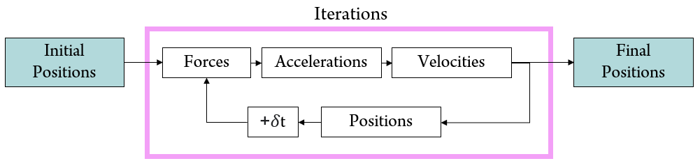
Figure 1. Numerical integrators solve for new atomic positions by iteratively calculating the system's interatomic forces, accelerations, and velocities.
Choosing an optimal integration time step δt is very important. If δt is too small (Figure 3), the number of steps required to finish the simulation would be too large. If δt is too large (Figure 4), the simulation is likely to diverge. An optimal δt models the dynamics accurately (minimizing algebraic errors) while keeping computational cost as low as possible (See Figure 2). In MD, the time step is often chosen to be at least an order of magnitude smaller than the fastest timescale in the system. In most cases, it is chosen empirically by trial and error as many system properties are affected by choosing a different δt (e.g., internal energy). For simple MD simulations (e.g., liquid Argon using the Lennard-Jones potential) typical δt values range from 0.5 to 2 fs.

Figure 2. An optimal δt means that there is a balance between the number of steps required to solve for new particle positions and how well the system is still represented. Notice how the particles do not overlap during the collision and depart away from each other smoothly.

Figure 3. A very small δt would result in more accurate results, but requires more steps. With MD simulations already being computationally expensive (even by today's standards), it is important to increase the value of δt to decrease computational cost.

Figure 4. Choosing a large δt would cause the integrator to place particles too close or too far from each other (e.g., overlapping them), often diverging the system. Notice how the particles overlap as a result of their position being calculated too far from their previous one, causing them to repel each other strongly and increasing the energy of the system unexpectedly.