numerical-methods-3 | Scymol project

Limiting the potential's range to a finite distance can be achieved in different ways. The easiest option is to simply imply that if the interatomic distance between atoms i and j, $r_{ij}$, is larger than a set distance, $r_c$, then the interatomic potential $E$ is equal to zero. This form of truncation is referred to as a Radial cutoff. $$ E\left(r_{ij}\right) = \begin{cases} E\left(r_{ij}\right)\ \ \ \ \ \ \ \ \ \ \ \ \ \ \ \ \ \ \ \ \ \ \ \ if\ \ r_{ij}< r_c\\ 0\ \ \ \ \ \ \ \ \ \ \ \ \ \ \ \ \ \ \ \ \ \ \ \ \ \ \ \ \ \ \ \ \ if\ \ r_{ij}\geq r_c\\ \end{cases} $$

**Figure 1.** Lennard-Jones potential being truncated by a Radial cutoff method at a distance of $~2.5σ$. The energies/forces beyond a distance *$r_c$* are discarded.

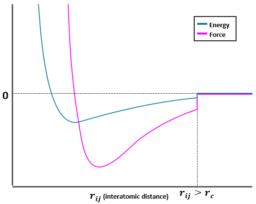
Potential truncation methods often introduce energy/force conservation problems, as there is an energy portion (even if small) being abruptly neglected at every integration step (see Figure 1). Another option known as the Cut and Shift method smoothens these energy interruptions so that the system better conserves energy/forces when $r_{ij} < r_{c}$. $$ E\left(r_{ij}\right) = \begin{cases} E\left(r_{ij}\right)\ -\ E\left(r_c\right)\ \ \ \ \ \ \ \ \ if\ \ r_{ij}< r_c\\ 0\ \ \ \ \ \ \ \ \ \ \ \ \ \ \ \ \ \ \ \ \ \ \ \ \ \ \ \ \ \ \ \ \ if\ \ r_{ij}\geq r_c\\ \end{cases} $$

Regardless of the truncation method applied, there is still the need to compute the interatomic distances between any atoms i and j, meaning that there are still ~$N^2$ evaluations to be computed.

Example

Velocities Verlet

A fully working example using the Velocities Verlet method is presented in Code 1. The code is simplified for readability and differs substantially from the one included in the source code of Scymol.

subroutine Verlet_Integrator()
!N is the total number of particles. 
!Px, Py, Pz, Vx, Vy, Vz, Ax, Ay, Az are the positions, velocities, 
!and acceleration arrays of the particles. 
!m is the mass array of the particles.
!dt is the integration time step. 
!boundary_conditions() calls a subroutine that updates the particles' 
!positions if they reach the boundaries.
!estimate_forces() calls a subroutine that evaluates the forces based 
!on the updated particles' positions and returns the 
!updated accelerations arrays. 

integer :: atom_i

!Verlet Estimator:
do atom_i = 1, N
    Vx(atom_i) = Vx(atom_i) + Ax(atom_i) * dt / 2
    Vy(atom_i) = Vy(atom_i) + Ay(atom_i) * dt / 2
    Vz(atom_i) = Vz(atom_i) + Az(atom_i) * dt / 2
    Px(atom_i) = Px(atom_i) + Vx(atom_i) * dt
    Py(atom_i) = Py(atom_i) + Vy(atom_i) * dt
    Pz(atom_i) = Pz(atom_i) + Vz(atom_i) * dt
end do

call boundary_conditions()
call estimate_forces()

!Verlet Propagator:
do atom_i = 1, N
    Vx(atom_i) = Vx(atom_i) + Fx(atom_i) * dt / 2 / m(atom_i)
    Vy(atom_i) = Vy(atom_i) + Fy(atom_i) * dt / 2 / m(atom_i)
    Vz(atom_i) = Vz(atom_i) + Fz(atom_i) * dt / 2 / m(atom_i)
end do
end subroutine Verlet_Integrator

Code 1. Pseudocode of a Velocities Verlet integrator estimating new atomic positions after one integration step.

3/3