Theoretical background
Potentials
The following section explains how potentials are used in Molecular Dynamics (MD) to update atomic positions in cartesian coordinates.
Background
MD methods calculate the positions, velocities, and accelerations of particles or atoms in a chemical system by using an integrator to solve the Newtonian equations of motion under the influence of specified force fields. Force fields are often derived from potential energy functions which represent the total energy of the system for a specific geometric arrangement of the particles in space. Force fields can be obtained (1) from literature. (2) by using smaller, more conservative MD simulations to estimate parameters that later can be applied to larger systems. (3) by using semi-empirical quantum mechanical approximations to estimate electrostatic potential maps and deriving the forces in place. (4) by calculating the electronic structure of a system using quantum mechanical calculations. Evidently, the last two options are the most time-consuming. The best force fields are often the ones that accurately model the system in study while being computationally efficient (easily solvable; the least time-consuming).
Potentials are often expressed in terms of energy (\(E\)) and they have to be converted into their force form to solve the Newtonian equations of motion in cartesian coordinates. This is achieved by differentiating the potential energy expression (\(E\)) with respect to the particle positions in the x, y, and z coordinates. $$F=-\nabla E\left(r\right)=-\frac{\partial E}{\partial r}$$ Manually deriving the expressions usually becomes a tedious task, especially for angular or torsional forces. However, with the aid of Sympy Python's Sympy library: https://pypi.org/project/sympy/ https://doi.org/10.7717/peerj-cs.103. , it is possible to symbolically differentiate these expressions with ease. Sympy is embedded into Scymol so that the potential energy expressions (\(E\)) entered by user are seamlessly differentiated, simplified, and introduced into the solver algorithm when a simulation is executed.
The energy expressions typed in by the user are grouped into five different categories of interaction potentials, as seen in Table 1.
Table 1. The five categories of potential energy functions that can be entered in Scymol. The user enters algebraic expressions similar to the ones shown as examples in the table. These examples are for expressions of potential energy interactions commonly used in MD simulations.
| Category |
Description | Illustration | Example | Interaction potential example |
|---|---|---|---|---|
| 1 | Force that is exerted on every particle. | 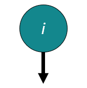 |
Gravity | $$E_i=g\sum_{i}^{N}m_i∆h$$ |
| 2 | Interaction force that affects two particles at a distance, regardless if they are bonded or not. |
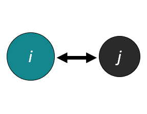 |
Van der Waals |
$$E_{i,j}=\sum_{i}^{N}\sum_{i\neq j}{4\epsilon_{ij}\left[\left(\frac{r_{ij}}{\sigma_{ij}}\right)^{-12}-\left(\frac{r_{ij}}{\sigma_{ij}}\right)^{-6}\right]}$$ |
| 3 | Interaction force between two particles that are bonded. |
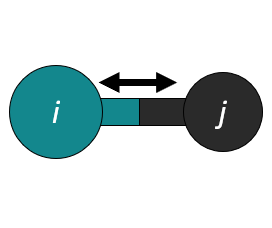 |
Harmonic bonding |
$$E_{i,j}=\sum_{i}^{N}{b_{ij}\times\left(r_{ij}-b_0\right)^2}$$ |
| 4 | Interaction force between three bonded particles forming an angle. |
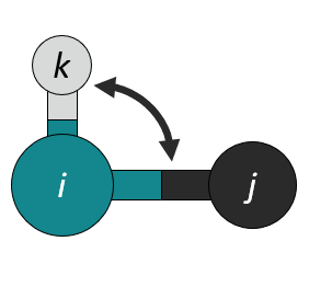 |
Harmonic angular |
$$E_{i,j,\ \ k}=\sum_{i}^{N}{a_{i,j,k}\times\left(\theta_{i,j,k}-\theta_0\right)^2}$$ |
| 5 | Interaction force between four particles forming a dihedral angle. |
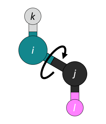 |
Harmonic torsional |
$$E_{i,j,\ \ k,l}=\sum_{i}^{N}\sum_{1}^{M}{t_{i,j,k,l}\left[1+cos{\left(M\emptyset_{i,j,k,l}\omega_{i,j,k,l}+\ \gamma_{i,j,k,l}\right)}\right]}$$ |
Example.
The Lennard-Jones potential (with 6 and 12 exponents) is given by $$ E_{i,j}=\sum_{i}^{N}\sum_{i\neq j}{4\epsilon_{ij}\left[\left(\frac{r_{ij}}{\sigma_{ij}}\right)^{-12}-\left(\frac{r_{ij}}{\sigma_{ij}}\right)^{-6}\right]} $$ The expression should be typed into Scymol in its energy form (following Fortran's expressions syntax) as a Type 2 interaction potential (see Table 1):
4*eps*((sigma/r)**12-(sigma/r)**6)
When a simulation is executed, Scymol (with the aid of Sympy) simplifies the expression (if possible): $$\frac{4\epsilon {\sigma}^6 \left(-\left(r^6\right)+{\sigma}^6\right)}{r^{12}}$$ Then, it proceeds to differentiate the expression with respect to \(r\): $$\frac{24\epsilon {\sigma}^6 \left(r^6-2{\sigma}^6\right)}{r^{13}}$$ Then, Scymol introduces and combines this force expression with the chain-rule derivatives relating \(r\) to the particles positions in x, y, and z coordinates: $$\frac{24\epsilon {\sigma}^6 \left(r^6-2{\sigma}^6\right) \left(x-x0\right)}{r^{13} \sqrt{{\left(x-x0\right)}^2+{\left(y-y0\right)}^2+{\left(z-z0\right)}^2}}$$ Resulting (for example) in the final expression responsible for estimating the force acting on particle i on the x coordinate: $$F_{x_i}=-24\varepsilon\sigma^6({r_{ij}}^{-7}-2\sigma^6{r_{ij}}^{-13})\frac{x_i-x_j}{\sqrt{\left(x_i-x_j\right)^2+\left(y_i-y_j\right)^2+\left(z_i-z_j\right)^2}}$$