units-example-2 | Scymol project

Example 2.

Let us assume we are setting up a simulation using an *.xyz file containing the atomic positions for a liquid Argon (Ar) system. The objective is to run an MD simulation and measure the kinetic temperature of the system. By default, xyz files have atomic coordinates expressed in angstroms ($Å$) thus making it the unit that measures length or distance in our system. We then proceed to input the atomic mass of our Ar atoms in Daltons ($Da$), where $m_{Ar}=39.948 Da$). We use ($Da$) because in computer simulations it is better to work with magnitudes close to the number 1 ($1×10^{-4} < x_i < 1×10^4$) to prevent loss of significance effects. If we were to use the Kilogram ($Kg$) instead of the Dalton ($Da$) we would be entering numbers in the range of ~$1×10^{-26}$.
The system's forces are computed using the Lennard-Jones potential: $$ E\left(r_{ij}\right)=4\epsilon_{ij}\left[\left(\frac{r_{ij}}{\sigma_{ij}}\right)^{-12}-\left(\frac{r_{ij}}{\sigma_{ij}}\right)^{-6}\right], $$ In Example 1 we had to convert the inputs to our units of choice ($g → 9.81 m/s^2$); we do the same here. Notice how the Lennard-Jones potential has two input parameters: $ε_{ij}$ and $σ_{ij}$. $σ_{ij}$ measures distance. We have already defined that distances in our system are measured in $Å$. $ε_{ij}$ measures energy $E$. Energy is a derived quantity equivalent to the following base quantities:

$$E=\frac{l^2m}{t^2}$$ where $l$ is length (already defined in $Å$), $m$ is mass (already defined in $Da$), and $t$ is time. Notice how we still need to define which unit is going to be used to measure time. It is customary to use the picosecond ($ps$) in MD because it produces results with magnitudes within $1×10^{-4} < x_i < 1×10^4$ when used in combination with the $Å$ and the $Da$. If we want to calculate the kinetic temperature of the system using the following relation: $$T_{kinetic}=\frac{2\bar{K_E}}{3k_b}$$ where $\bar{K_E}$ is the kinetic energy of the particles and $k_b$ is the Boltzmann constant, we would have to define the unit to measure temperature ($T$) as well. We can use the Kelvin ($K$) and make sure to convert $k_b$ to the system of units that we have defined until now. $k_b$ would be equal to $0.831036 Å^2Da/{ps^2K}$.
In conclusion, our custom system of fundamental units selected for this example is defined by: the angstrom $Å$ to measure length, the Dalton $Da$ to measure mass, the picosecond $ps$ to measure time, and Kelvin $K$ to measure temperature. Any quantity inputted into Scymol would have to be converted to this system of units. In return, any quantity returned by Scymol will be based on this unit system. For example, the velocities of the particles would be measured in $Å/{ps}$, acceleration in $Å/{ps^2}$, force in $mÅ/{ps^2}$, energy in $mÅ^2/{ps^2}$, and temperature in $K$. A conversion list from this system of units to SI is found in Table 2 (page 1). Post-processing tools included in Scymol would output quantities that rely on these custom units as well, as seen in Figure 1.

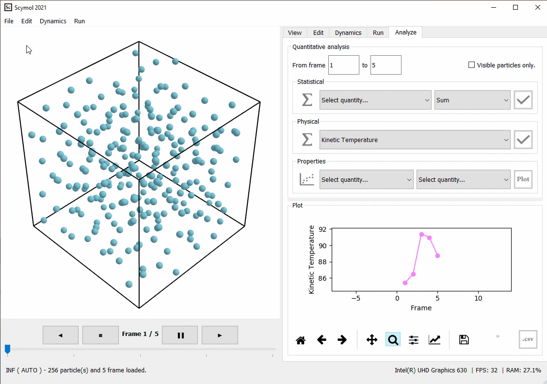
**Figure 1.** The average kinetic temperature of the system of liquid argon is computed by Scymol and is equal to $88 K$. Notice how Scymol displays 88, but not because the tool is programmed to automatically compute temperature in Kelvin ($K$) but because the combination of the quantities necessary to estimate the kinetic temperature produce a number measured in ($K$), as established by our choice of fundamental units.

3/4