Type 5 forces
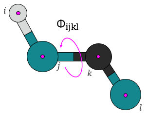
Figure 1. This force category includes forces that result from the torsional strain generated by four consecutive bonded atoms i, j, k, and l forming a dihedral angle (\(\phi_{i,j,k}\)).
The total energy \(E_{Type \ \ 5}\) of the system at any given time is given by the summation of the energies present at each dihedral angle(\(\phi_{i,j,k}\)) formed by atoms i, j, k, and l (see Figure 1). $$E_{Type\ 5}=\sum_{i,j,k,k}^{Torsional\ quads}E_{i,j,k,l},$$ where \(E_{i,j,k,l}\) is the energy resulting from the formation of a torsional strain between four bonded atoms i-j-k-l.
Figure 2. The dihedral quads are generated by Scymol by searching for chains of four atoms. Notice how atoms that do not form an atomic quad are omitted.
Even though the calculation of the resulting forces (and thus, the resulting particle positions) due to the presence of dihedral (or torsional) strains is considerably harder than every other force type (2, 3, and 4), the number of atomic quad usually grows with (\(~N\)) in common chemical systems (see Figure 2). This means that estimating dihedral strain effects on MD systems is computationally inexpensive.
Torsional potentials often rely on applying a torsional strain on particles i, j, k, and l if the dihedral angle formed (\(\phi_{i,j,k}\)) is not very close to some reference angle (\(\phi_{(i,j,k),0}\)). If the potential has several equilibrium angles, it is said that the potential has a multiplicity equal to \(m\). In that case, the energy of the system is given by: $$E_{Type\ 5}=\sum_{1}^{m}\sum_{i}^{bonded\ quads}E_{(i,j,k,l),\ \ \ m},$$ where \(E_{i,j,k,l}\) is the energy contribution of each bonded atomic quad i-j-k-l and \(m\) is the multiplicity of the potential. Due to the different conformations that many molecules can take, torsional potentials usually have multiple (\(m\)) reference (or equilibrium) angles (\(\phi_{(i,j,k),m}\)). For example, ethane has 6 notable conformations (3 eclipsed and 3 staggered). This means that torsional potentials that model ethane often have a multiplicity \(m = 6\).
Example 1.
Many modifications are found in literature. In fact, torsional forces are often modelled using a Harmonic potential (just like in the case of forces of types 3 and 4) but with multiple equilibrium positions and thus a multiplicity larger than one (\(m>1\)). This is why the potentials used to model torsional forces are often expressed as a Fourier series summation so that every equilibrium position is modelled with the algebraic expression used.
Here, we show how the position of a particle i is updated by Scymol's solver
using a torsional potential (refer to Figure 2). Note that not all the particles are affected in similar ways; the formulae used for particle i are different from those used for particles j, k, and l.
$$\frac{\partial E_t}{x_i}=\frac{\partial E_t}{\partial\phi_{ijkl}}\ \frac{\partial\phi_{ijkl}}{\partial \theta_{1,2,3}} \frac{\partial\theta_{1,2,3}}{\partial x_{i}}$$
The following algebraic calculations are performed to calculate the effect of the torsional potential on particle i in the x-coordinate:
First, we define the points and vectors used throughout the calculations given that we have four points containing the positions of atoms i, j, k and l:
$$P_{(x,kj)}=P_{(x,k)}-P_{(x,j)}$$
$$P_{(x,ij)}=P_{(x,i)}-P_{(x,j)}$$
$$P_{(x,lk)}=P_{(x,l)}-P_{(x,k)}$$
$$P_{(y,ij)}=P_{(y,i)}-P_{(y,j)}$$
$$P_{(y,kj)}=P_{(y,k)}-P_{(y,j)}$$
$$P_{(y,lk)}=P_{(y,l)}-P_{(y,k)}$$
$$P_{(z,lk)}=P_{(z,l)}-P_{(z,k)}$$
$$P_{(z,kj)}=P_{(z,k)}-P_{(z,j)}$$
$$P_{(z,ij)}=P_{(y,i)}-P_{(z,j)}$$
Then, we proceed to compute the vectors normal to the intersecting planes formed by the points i, j, k and j,k,l:
$$N_{(1,x)}=P_{(y,ij)} P_{(z,kj)} - P_{(z,ij)} P_{(y,kj)}$$
$$N_{(1,y)}=P_{(z,ij)} P_{(x,kj)} - P_{(x,ij)} P_{(z,kj)}$$
$$N_{(1,z)}=P_{(x,ij)} P_{(y,kj)} - P_{(y,ij)} P_{(x,kj)}$$
$$N_{(2,x)}=P_{(y,lk)} P_{(z,kj)} - P_{(z,lk)} P_{(y,kj)}$$
$$N_{(2,y)}=P_{(z,lk)} P_{(x,kj)} - P_{(x,lk)} P_{(z,kj)}$$
$$N_{(2,z)}=P_{(x,lk)} P_{(y,kj)} - P_{(y,lk)} P_{(x,kj)}$$
We continue by estimating some input parameters used by the partial derivatives:
$$\sigma=sign((\vec{P_1P_2}x\vec{P_3P_2})\bullet(\vec{P_4P_3}))$$
$$\cos{\left(\phi_{ijkl}\right)}=angle(N_1,O,N_2)$$
$$\phi_{ijkl}=\arccos{\left(\cos{\left(\phi_{ijkl}\right)}\right)}$$
$$L_1=\sqrt{N_{1,x}^2+N_{1,y}^2+N_{1,z}^2}\ \ $$
$$L_2=\sqrt{N_{2,x}^2+N_{2,y}^2+N_{2,z}^2}$$
$$A=dot\left(N_1,N_2\right)$$
$$B=-\frac{1}{\sqrt{1-L_1^2L_2^2\cos^2{\left(\phi_{ijkl}\right)}}}$$
Then we proceed to calculate the partial derivatives in x (Notice that in this part we are applying the same method used in forces of type 4):
$$\frac{\partial\theta_{1,2,3}}{\partial x}=B\left(L_1L_2\left(N_{1,x}\right)-A\frac{L_2}{L_1}\left(N_{2,x}\right)\right)$$
$$\frac{\partial\theta_{1,2,3}}{\partial y}=B\left(L_1L_2\left(N_{1,y}\right)-A\frac{L_2}{L_1}\left(N_{2,y}\right)\right)$$
$$\frac{\partial\theta_{1,2,3}}{\partial z}=B\left(L_1L_2\left(N_{2,z}\right)-A\frac{L_2}{L_1}\left(N_{2,z}\right)\right)$$
We then estimate the final relationship between the dihedral angle and the position of atom i in the x-coordinate:
$$\frac{\partial\phi_{ijkl}}{\partial P_{x,i}}=\sigma\left(\frac{\partial\theta_{1,2,3}}{\partial y}\left(P_{z,j}-P_{z,k}\right)+\frac{\partial\theta_{1,2,3}}{\partial z}\left(P_{y,k}-P_{y,j}\right)\right)$$
We estimate the derivative of our energy function (without any chain rule terms):
$$\frac{\partial E_{ijkl}}{\partial\phi_{ijkl}}=\sum_{1}^{m}{2t_{i,j,k,l}\times(\phi_{ijkl}-\emptyset_0)}$$
And finally, we combine the partial derivatives into one expression: