Type 3 forces
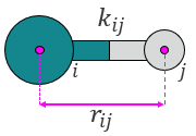
Figure 1. This force category includes forces that result from the strain caused by the stretching or compressing of the bond that exists between atoms i and j distanced \(r_{ij}\) units apart.
This subdivision includes attractive and/or repulsive forces between particles i and j that are physically bonded (see Figure 1). The total energy \(E_{Type\ \ 3}\) of the system at any given time is given by the summation of the energies present between each bonded atoms in the system (see Figure 2). $$E_{Type\ 3}=\sum_{i}^{bonded\ \ pairs}\sum_{i\neq j}^{N}E_{i,j},$$ where \(E_{i,j}\) is the energy between the bonded atoms i-j.
Figure 2. The two bonded atoms are generated by Scymol by searching for every particle i that is bonded to another atom j. Notice how atoms that do not form a bond are omitted. Duplicate pairs (i.e., bond pair i,j and j,i) are omitted, as the force is considered to be equal in magnitude but with opposite sign to the one evaluated already for the previous pair.
The number of bonded atoms usually grows with (\(~N\)) meaning that estimating bonding strain effects on MD systems is computationally inexpensive when compared to when estimating forces of type 2 (see Figure 2).