potentials-type-2 | Scymol project

Type 2 forces

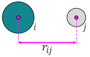
**Figure 1.** This force category includes forces that result from the interaction of every non-bonded atoms i and j distanced $r_{ij}$ units apart.

This subdivision includes attractive and/or repulsive forces between particles i and j that share no bonds. The total energy $E_{Type\ \ 2}$ of the system at any given time is given by the summation of the energies present between every two atoms in the system (see Figure 1). $$E_{Type\ 2}=\sum_{i}^{N}\sum_{i\neq j}^{N}E_{ij},$$ where $E_{i,j}$ is the energy between the atoms i-j.

**Figure 2.** Every atom i interacts with every other atom j in the system. Repeated pairs are shown in the GIF (e.g., *i-j* and *j-i*), however, most solvers use one atomic pair, and assume the other pair's force to be of the same magnitude but with opposite sign to save computation time.

The computational time required to evaluate the force for every atomic pair is by far the longest in an MD sequence. The number of atomic pairs in a system of particles is given by $N\times(N-1)$, which tends to $~N^2$ when $N$ is large enough (see Figure 2). Most of the optimization done in MD calculations is focused on how to efficiently evaluate the interactions of this force type. Moreover, it is common to see systems that neglect the effects of forces of type 3, 4, and 5, but seldom (if ever) the interactions of forces of type 2. Many workarounds exist to reduce the number of force evaluations, and often take advantage of the following points:
•Forces are set to zero beyond a distance $r_{ij}>r_{cut}$, so that the force calculation for that specific pair is skipped.
•Generating the atomic pairs at each integration step is often not necessary, and so updating this pairs list is done on more separate intervals. This is known as a neighbors list and/or a Verlet list. If properly applied, this method can decrease the number of force evaluations to $~N$ rather than $~N^2$.
•The MD code can be made to run in a parallelized manner so that the force evaluation work is divided among several CPU cores.
Scymol allows the user to define an $r_{cut}$, an update list interval, and the number of cores desired so that the MD code is distributed among several CPU cores.

Example 1.

In the following example, we convert an energy potential ($E$) into its force form and we explain how the solver calculates the new particle position from this force. A common potential in this category is the Lennard-Jones potential used to model Van der Waals interactions. The Lennard-Jones potential is given by: $$ E_{i,j}=\sum_{i}^{N}\sum_{i\neq j}{4\epsilon_{ij}\left[\left(\frac{r_{ij}}{\sigma_{ij}}\right)^{-12}-\left(\frac{r_{ij}}{\sigma_{ij}}\right)^{-6}\right]} $$ Notice how these interactions depend entirely on the distance $r_{ij}$ between the particles.
Differentiating this expression to get the force with respect to the position of particle i in the x-coordinate yields: $$F_{i,x}=-\frac{\partial E}{\partial r_{ij}} \frac{\partial r_{ij}}{\partial x_i}$$ The resulting expression is computed using SymPy's differentiation function sympy.diff(str_energy_expression): Expression was manipulated for readability.
SymPy's diff function: https://docs.SymPy.org/latest/tutorial/calculus.html. $$F_{x_i}=-24\varepsilon\sigma^6({r_{ij}}^{-7}-2\sigma^6{r_{ij}}^{-13})\frac{x_i-x_j}{\sqrt{\left(x_i-x_j\right)^2+\left(y_i-y_j\right)^2+\left(z_i-z_j\right)^2}}$$ The same has to be done for the remaining coordinate positions and for particle j as well. Plotting the energy ($E$) and force ($F$) against interatomic distance ($r_{ij}$) is seen in Figure 3.

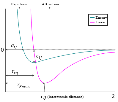
**Figure 3.** Attractive-repulsive nature of the Lennard-Jones potential modeling Van der Waal interactions. Small changes in interatomic distance result in huge energy shifts due to the large exponents of the Lennard-Jones algebraic expression (6 and 12). Particles that are initially positioned too close to each other, integration steps that are too large, or unrealistic changes introduced into the system can easily cause the particles to *explode*, and thus causing the solver to diverge.

Example 2.

Electrostatic (or Coulomb) interactions are another example of pairwise interactions that occur between non-bonded atoms. This time, the atoms i and j hold electric charges.

These charges generate an electrostatic potential around the atoms that decays with interatomic distance. The potential is modeled by the following expression: $$E\left(r_{ij}\right)=\frac{q_i q_j}{4\pi\epsilon_0r_{ij}},$$ where $q_i$ and $q_j$ are the atomic charges for atoms i and j, $\epsilon_0$ is the vacuum permittivity constant, and $r_{ij}$ is the interatomic distance. Again, SymPy's 'diff' function is used to estimate the resulting force expression that acts on both atoms in cartesian coordinates. The function results in the following expression of the force acting on particle i on the x-cordinate. 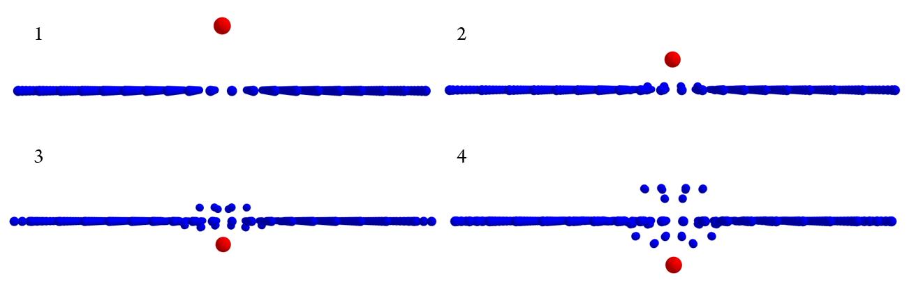$$F_{x_i}=-\frac{-q_iq_j}{4\pi\epsilon_0\epsilon_Rr_{ij}^2}\frac{x_i-x_j}{\sqrt{\left(x_i-x_j\right)^2+\left(y_i-y_j\right)^2+\left(z_i-z_j\right)^2}},$$ where $q_i$ and $q_j$ are the atomic charges for atoms i and j, $\epsilon_{0}$ is the vacuum permittivity constant, $r_{ij}$ is the interatomic distance, and $x$, $y$, $z$ are the atomic positions for atoms i and j. Figure 4 presents a 'textbook' example of a surface of negatively charged particles being affected by a single positively charged particle at a distance.

**Figure 4.** The influence of one particle over another depends on the distance between them. Notice how negatively charged particles right below the positively charged one are immediately affected.

2/5