numerical-methods-2 | Scymol project

Boundary Conditions

Boundary conditions refer to what happens to the particles when they reach the limits of the simulation box. Scymol includes by default a number of different conditions:

●Bounce
●Wraparound
●Periodic Boundary Conditions (PBC)
●Stop
●No boundaries

We are going to explain PBC due to their relevance in MD.
In MD simulations, the presence of invisible boundaries that define the simulation box (i.e., walls) has a significant influence on how well the simulation resembles a system of macroscopic dimensions. The number of particles N present in a simulated system is almost always negligible when compared to macroscopic quantities (in the order of \(N \approx 10^{22}\)). MD simulations rarely surpass \(N\approx 10^7\) particles, even when run on the largest computer clusters available today. Moreover, in macroscopic systems, only one in about ten million particles are considered surface atoms.
This means that computer simulations with necessarily small Ns have to overcome the effects of boundary dynamics to successfully recreate a macroscopic system. The most convenient solution to overcome these issues is to use PBC, where the initial system is replicated an infinite number of times in every dimension to simulate an 'infinitely' large system. This effectively removes boundary effects, and allows simulations of just a few hundred Ns to successfully estimate properties of bulk systems of macroscopic proportions. See Figure 1 to see how PBC are applied into a simulation box with \(N\) particles.

**Figure 1.** In MD, **PBC** are used to virtually eliminate surface effects while having a finite, but unbounded region. Particles that leave from one side reappear from the other side with the same speed and trajectory. Particles also interact with other particles from the box itself or from image particles beyond the boundaries. Notice how a particle close to the boundary affects another particle on the opposite side of the wall.

Code 1 is a pseudocode example showing how PBC are usually programmed in computer simulations (taking into account the x-coordinate only).

!Definitions:
!N = number of atoms. 
!Px = atomic positions.
!dt = Integration step.
!dx = distance between atoms i and j.
!Lx = simulation's box side length.
!x1, x2 = boundary extremes. 

!Velocities Verlet Predictor:
Vx = Vx + Ax * dt/2
Px = Px + Vx * dt

call Forces()
call BoundaryConditions()

!Velocities Verlet Corrector:
Vx = Vx + Ax * dt/2

subroutine Forces()
do i = 1, N - 1
    do j = i + 1, N
	dx = Px(i) - Px(j)
	if (abs(dx)>0.5*Lx) then
	    dx = dx - sign(Lx, dx)
	end if
	!calculateForces with dx.
end subroutine Forces

subroutine BoundaryConditions()
do i = 1,N
    if (Px(i) > x1) then
	Px(i) = x2
    elseif (Px(i) < x2) then
	Px(i) = x1
    end if
end do
end subroutine BoundaryConditions

Code 1. There are two parts that must be added into the general code. First, the interatomic distance needed to calculate the acting forces has to take into account particles beyond the boundaries. Second, particles must reappear on the opposite side if they cross the walls, replicating a 'wraparound' effect. In the pseudocode, these modifications are added into the Forces() and the BoundaryCondition() subroutines.

Potential Truncations

The most time-consuming section of most particle simulations corresponds to estimating pairwise interactions at every integration step. In this type of interaction, each particle i interacts with every other particle j. This means that the number of interactions required to compute pairwise interactions in a system of N particles approaches ~\(N^2\). The use of PBC (or similar methods that try to mimic infinitely large systems) forces one particle to interact with all the other particles within its own box, and infinite copies of this box. This means that in theory, the number of interactions would approach infinity even if only one particle is considered. Therefore, workarounds must be applied to reduce the number of considered interactions.
The most commonly used solution is to set a maximum interaction distance for each particle, beyond which the potential is set to zero. In other words, the interatomic potential is limited to a finite range. In MD, this proves to be very useful in reducing the number of computations because it effectively eliminates the 'infinite' interactions problem that arises from using PBC and because most of the pairwise potentials (e.g., Lennard-Jones) tend to zero at very short interatomic distances.

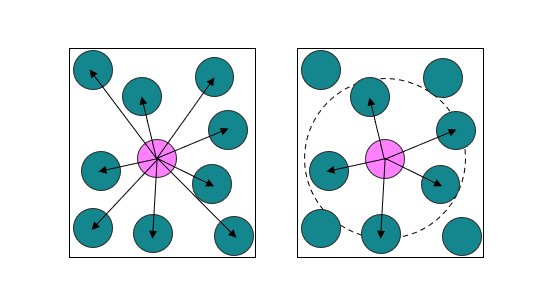
**Figure 2.** A commonly used technique to save up computational costs is to limit the range of the potential to a finite interatomic distance, beyond which it is set to zero. Notice how the number of interactions is cut by half in the simulation to the right. If the Lennard-Jones potential were to be applied, the force that is being discarded in the simulation accounts for only 0.7% of the total force acting on the highlighted particle.

2/3