Section 4. Measuring transport properties
We are going to follow these steps in order to estimate \(D\), \(η\), \(C_v\), and \(k\)
• Estimate the Mean Squared Displacement (\(MSD\)).
• Compute the self diffusivity coefficient (\(D\)).
• Calculate the viscosity (\(η\)) of liquid Argon using the value of (\(D\)).
• Calculate the thermal conductivity (\(k\)) from the value of \(η\) obtained.
• Estimate the heat capacity (\(C_v\)) by inducing a change in the system's temperature and computing the change in the system's energy.
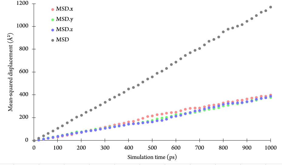
Figure 1. The Mean-squared displacement is plotted against the simulation time. The particles diffuse nomrally (i.e., plot's slope is close to one) with respect to time. If your simulation's MSD values are different, or if your plot's slope is evidently larger or smaller than one, it means that your simulation was not properly initialized or run for long enough so that the particles reach a proper equilibrium before measuring the MSD.
The dynamic viscosity of liquid argon can be approximated using Li and Chang’s Li and Chang’s modification to the Sutherland formula, that correlates the self-diffusivity constant (\(D\)) with dynamic viscosity \(η\) in homogenous liquids. https://doi.org/10.1063/1.1742022 modification to the Sutherland formula, that correlates the self-diffusivity constant (\(D\)) with dynamic viscosity \(η\) in homogenous liquids (like pure liquid Argon) organized in a perfect cubic cell. The approximation is given by: $$\eta=\frac{K_bT}{2\pi D}\left(\frac{N_{av}}{V}\right)^\frac{1}{3},$$ where \(k_b\) is the Boltzman constant, \(T\) is the system's temperature, \(D\) is the self-diffusivity coefficient, \(N_{av}\) is Avogadro's number, and \(V\) is the volume of the system. The computed value for \(η\) is $$η \approx 2.8 \times 10^{-4}$$ which compares well with the reported value of \(η_{theoretical}=2.7 \times 10^{-4}\).
The isochoric heat capacity (\(C_v\)) can be approximated by applying the fluctuation dissipation theorem to measure the instantaneous thermal and energy fluctuations that occur in the simulation of Stage 3 (i.e., a constant N, V, and E simulation) at equilibrium. Therefore, we do not need to run another simulation to induce a temperature change to estimate the heat capacity of our system. The fluctuation dissipation theorem to measure heat capacity in an NVE system at equilibrium is given by $$\left \langle K_e^2 \right \rangle - \left \langle K_e \right \rangle^2 = \frac{3Nk_b^2T^2}{2}\left(1-\frac{3Nk_b}{2C_v}\right) ,$$ where \(K_e\) is the kinetic energy, \(N\) is the number of particles, \(k_b\) is the Boltzmann constant, and \(T\) is the average kinetic temperature. Go into the Analyze tab, enter a range that includes only steps from Stage 3, and select the NVE - Isochoric Heat Capacity (in the Physical Quantities option). The computed \(C_v\) should be close to: $$C_v \approx 1.6 E/K/atom$$ If you need more accurate values for \(C_v\), you would need to either increase the number of particles, make sure the system is properly equilibrated at 85 K, or run a longer simulation.
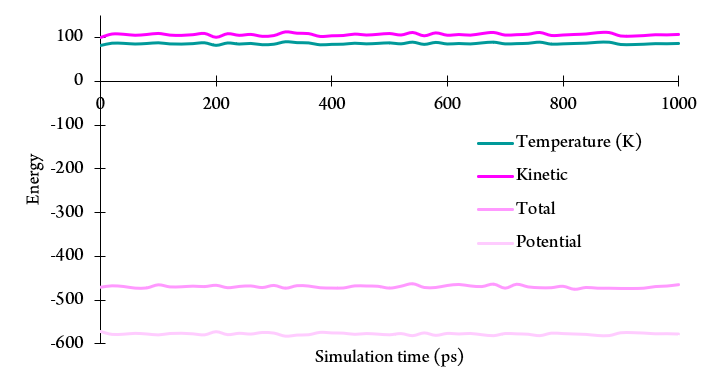
Figure 2. There are small energy fluctuations even though the system is at equilibrium. These fluctuations can be used to measure the isochoric heat capacity by measuring the variance of our energy and temperature values and applying the fluctuation dissipation theorem.
The thermal conductivity \(k\) is estimated using the Andrade's Andrade's relationship between the \(η\) and \(k\) in monoatomic saturated liquids. https://doi.org/10.1038/170794b0 relationship between the \(η\) and \(k\) for monoatomic saturated liquids: $$k=\beta\times\eta\times C_v,$$ where k is the thermal conductivity, \(\beta\) is an input parameter that depends on the nature of the system, \(η\) is the dynamic viscosity, and \(C_v\) is the isochoric heat capacity computed above. The computed value should be close to: $$k \approx 1.32 E/K/atom $$ which compares well to the reported values of thermal conductivity of liquid Argon.