Section 3. Production stage
Video 1. Section 2 summarized into a 1 minute video. For a detailed explanation, follow the tutorial below.
Before running the simulation, make sure you change the length of the simulation to '500' and make sure you leave the Number of simulations to run in series input box empty (or set to 1). The custom Python code will not be executed if the number of simulations to be run is equal to 1. After the simulation finishes, make sure that the system temperature is still around 85 K before proceeding into Section 4.
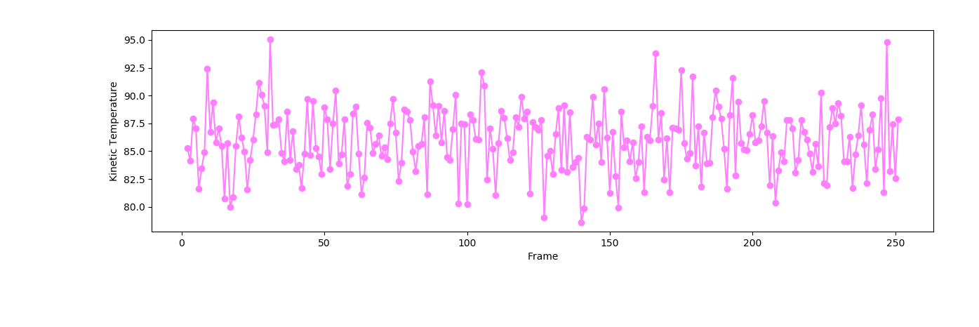
Figure 1. The instantaneous kinetic temperature at equilibrium should fluctuate around 85 K. Smaller fluctuations are expected on systems with a larger number of particles \(N\). Your system should behave similarly to the one shown in the figure. If your system is not stable at 85 K, make sure that you have equilibrated the system long enough before, during, and after any temperature control steps.